![]()
Frontline Learning Research Frontline Learning
Research Special Issue Vol.9 No.2 (2021) 121 - 144
ISSN 2295-3159
1Surrey Institute of Education,
University of Surrey, UK
Article received 18 May 2020/ revised 22 September / accepted 21 October/ available online 12 March
A significant challenge currently facing the higher education sector is how to address differential student outcomes in terms of attainment and continuation gaps at various stages of students’ transitions. Worryingly, there appears to be a ‘deficit’ discourse among some university staff in which differential outcomes are perceived to be due to student deficiencies. This may be exacerbated by institutional analyses placing an over-emphasis on the presence of the gaps rather than the causes. The purpose of this primer is to provide advice about how institutions can carry out far more nuanced analyses of their institutional data without requiring specialist software or expertise. Drawing on a multi-level framework for explaining differential outcomes, we begin with guidance for gathering quantitative data on explanatory factors for attainment and continuation gaps, largely by linking sources of internal data that have not previously been connected. Using illustrative examples, we then provide tutorials for how to model explanatory factors employing IBM SPSS Statistics (IBM Corp., Armonk, NY, USA) to perform and interpret regression and meta-regression analyses of individual- and group-level (aggregated) student data, combined with data on micro- and meso-level factors. We propose that university staff with strategic responsibilities could use these approaches with their institutional data, and the findings could then inform the design of context-specific interventions that focus on changing practices associated with gaps. In doing so, institutions could enhance the evidence-base, raise awareness, and further ‘embed the agenda’ when it comes to understanding potential reasons for differential student outcomes during educational transitions.
Keywords: diversity; transitions; attainment gaps; continuation gaps; micro, meso and macro level
Recent transitions research has signalled a move away from seeing students as a homogeneous group undergoing a ‘transition process’ to acknowledging the importance of their diversity as they progress through university (Gravett, 2019). One aspect of diversity that presents a significant challenge for the higher education sector relates to the presence of differential student outcomes. Whilst at university, students from underrepresented backgrounds generally have lower levels of achievement (known as attainment gaps), and are less likely to progress from one year to the next (known as continuation gaps), than their traditional counterparts (OfS, n.d.). Differential outcomes have been found for students from a range of backgrounds, with poorer attainment and continuation outcomes for those who are mature, studying part-time, from a lower socioeconomic group, and from a Black, Asian, and minority ethnic background (Woodfield, 2014). These gaps have been identified across the sector internationally, including in the UK, USA, Australia, Belgium, Germany, and Denmark (Lens & Levrau, 2020; Mountford-Zimdars et al., 2015; Singh, 2011; Tieben, 2020).
Despite prior attainment and type of entry qualification only partially accounting for the presence of gaps (Broecke & Nicholls, 2007), there appears to be a ‘deficit’ discourse among some university staff in which differential outcomes are perceived to be due to student deficiencies (Miller, 2016; Singh, 2011; Stevenson, 2012). This may be exacerbated by institutional analyses placing an over-emphasis on the presence of the gaps themselves. Universities routinely collect a range of quantitative data at the point of student enrolment, some of which is then utilised to assess whether their widening participation targets are being met. These data may include demographic details such as gender, age, ethnicity, disabilities, and socioeconomic group, and they are further used to model whether there are differential outcomes in terms of attainment or continuation gaps at various stages of students’ transitions (e.g. end of first year grades, when progressing from the first year to the second year, etc.). Analysing these data is necessary for regulatory reporting purposes, but these data alone do not aid teaching staff in their design of interventions for tackling the causes of these gaps. A recent report also highlighted this over-reliance on collecting quantitative data at the expense of engaging with students about their actual experiences (UUK & NUS, 2019).
Since differential student outcomes are quantitatively assessed (Jones, 2018), qualitative evidence alone cannot be used to ascertain the factors that explain why there are gaps. Institutions have a duty to both monitor and attempt to reduce gaps, so this is likely to be an important target for senior management. However, we argue that any large-scale quantitative analyses of attainment and continuation gaps need to move beyond solely focusing on the presence of the gaps, and characteristics of the students, to take into account the explanatory factors for these differential outcomes. In order for teaching staff to improve the focus and design of interventions addressing gaps, they need to know the precise factors that may impact on these outcomes for their own students, drawing on evidence from their own institutional and disciplinary contexts (Mountford-Zimdars et al., 2017). Thus, quantitative analyses may offer a way forward, but more nuance is likely to be needed when determining which data to analyse and how:
Universities need to take a more scientific approach to tackling the attainment gap, by gathering and scrutinising data in a far more comprehensive way than they may currently be doing, in order to inform discussions between university leaders, academics, practitioners and students. (UUK & NUS, 2019, p. 2)
Therefore, the purpose of the current primer is to provide accessible guidance on the decisions that institutions should consider making when attempting to draw on evidence for the factors that may explain differential student outcomes. This primer provides suggestions for how explanatory factors can be quantitatively collected, and most importantly, how these data can be analysed using relatively straightforward approaches that do not require access to specialist software or expertise. It provides tools to model potential factors explaining differential outcomes within specific contexts throughout students’ transitions. Such models could then be used to stimulate conversations between teaching staff and students around issues that have been identified, and enable the design of context-specific interventions that focus on changing practices that have been confirmed to be associated with gaps. This could also extend the literature on differential outcomes.
In his theory of student departure, Tinto (1993) asserts that student persistence is based on how well they integrate into the social and academic systems of their university. This ability to integrate is thought to be influenced by students’ background characteristics, the institutional environment, and their experiences and interactions whilst they are at university. Building on the findings of Cousin and Cuerton’s (2012) attainment gap report, Mountford-Zimdars et al. (2015) conducted a critical review of the potential causes of differential student outcomes to identify explanatory factors for outcome gaps, which they categorised into: Students’ experiences of curriculum practices; relationships between staff and students; social, cultural and economic capital; and psychosocial and identity factors. Mountford-Zimdars et al. also proposed the use of a multi-level framework for understanding these explanatory factors. At a micro-level, explanatory factors may be related to the individual student and their one-to-one interactions with university staff. At a meso-level, explanatory factors may involve institutional and learning environment factors. At a macro-level, explanatory factors may be due to the wider higher education context and structure. These explanatory factors intersect with the multi-level framework, so they may occur at multiple levels and at various stages throughout students’ transitions. Figure 1 shows how these explanatory factors might manifest at the multiple levels of Mountford-Zimdars et al.’s framework.

Figure 1. Multi-level framework of explanatory factors for differential student outcomes based on the model from Mountford-Zimdars et al. (2015)
Although institutions have attempted to tackle differential student outcomes, interventions often simultaneously target both micro- and meso-level components, so it is difficult for teaching staff to disentangle which actions are reducing gaps and which are unsuccessful (Miller, 2016). As a result, research-informed changes to practice may currently be limited. Incorporating the model in Figure 1 into quantitative analyses may enable a greater understanding of the specific aspects of students’ backgrounds and the university environment that are associated with differential outcomes within specific contexts. Mountford-Zimdars et al. (2015) made several recommendations for reducing differential student outcomes in their report, and we propose that the current primer might support institutions in attending to some of those suggestions. Firstly, this primer provides guidance about how to enhance the evidence-base by drawing on module-level data 1 , linking sources of internal data that have not previously been connected to increase understanding about the institution’s context within the larger national and international picture. The methods should raise awareness among staff with strategic responsibilities, enabling interventions to be informed by evidence that is relevant to the institutional context. Finally, this primer supports institutions in ‘embedding the agenda’ through aiding the design of both targeted interventions (i.e. interventions that are directed at specific student groups) and universal interventions (i.e. interventions for all students that may be particularly beneficial for specific student groups).
Since explanatory factors that occur at the micro- and meso-levels are perceived to be the institution’s responsibilities (Mountford-Zimdars et al., 2015), these factors need to be operationalised if they are to be included in quantitative models. Micro-level factors occur at an individual level, so it is possible to quantify some of these as variables using validated self-report questionnaires. For example, the University Attachment Scale (France et al., 2010) includes a subscale for measuring students’ sense of belonging to the university. Meso-level variables mostly involve the group-level features of modules and programmes. Whilst the potential difficulty of gathering quantitative data of curriculum content has previously been noted (Miller, 2016), we suggest that these data could be obtained from a document analysis or audit of module descriptors, module booklets, examiner reports, prospectuses, the VLE structure and use, etc. There is likely to be a wealth of data available that could be useful, covering support available to students, types of assessment, extra-curricular activities, departmental policies, and anything else that may be relevant to the disciplinary and institutional context. The use of learning analytics data might also prove useful at both micro- and meso-levels. Since macro-level variables occur at the sectoral level, it may be difficult to model variation in these variables unless data are being shared across institutions, but there is scope for gathering these data. Ultimately, each institution needs to identify their own priorities whilst ensuring they align with the discussed theory. They must base their priorities on the relevance of the variables to their particular student groups, the data they have available, and whether their documentation is an accurate depiction of actual practices and how they are received by students.
In this section we provide tutorials for how to perform and interpret analyses of institutional data that do not require any specialist knowledge beyond a basic understanding of statistics. All tutorials utilise IBM SPSS Statistics (IBM Corp., Armonk, NY, USA) and all SPSS data sets, syntax files and macros to run and adapt analyses for readers’ own purposes are freely available at https://doi.org/10.5281/zenodo.4115264, so readers only need access to SPSS software to perform the same analyses or adaptations of these2. Because SPSS syntax has been provided with code for all of the procedural steps of running the necessary statistical tests, we only focus on how to interpret the results of such analyses. The data for all examples in this primer are fictional, and have only been designed to simulate the possible behaviour of institutional data for the purposes of demonstrating how the analytical approaches can be used. No inferences or conclusions should be drawn from the findings of these examples, because the results are not real. We anticipate that readers can use the example data sets as templates and substitute in their own data.
If data for individual students (e.g. their demographic details and possibly questionnaire responses) are accessible for the purposes described in this primer, it is possible to analyse these data using two common regression approaches based on the General Linear Model (GLM). Therefore, in Tutorials 1 and 2 we provide guidance about how to perform and interpret analyses of example individual-level data in order to model potential explanatory factors as covariates 3 of attainment and continuation gaps. These examples focus on micro-level explanatory factors, because these occur at the individual level. The questions we aim to answer in these examples are: Are there attainment/continuation gaps based on the students’ background groups, and can a set of micro-level factors predict attainment/continuation over and above these groups?
We anticipate that there may only be access to aggregated data for analysis due to individual-level data being restricted to certain staff or because consent has not been obtained to connect sensitive student data to other variables, so in Tutorials 3 and 4 we cover how meta-regression can be used to analyse such data. Meta-analysis was designed to synthesise an average effect size and how much it varies across multiple studies (Pigott & Polanin, 2020). The GLM can be extended in meta-analysis to also model the role of study-level covariates in explaining effect sizes (Field & Gillett, 2010; Hedges et al., 2009). This is known as meta-regression. Therefore, we propose that differences in data averaged for particular student groups at a module-level can be treated as an effect size, with the overall programmes functioning in the same way that separate studies do in meta-analysis studies. Further, meso- and macro-level factors can be treated as study-level covariates because these occur at a module, programme, institution and sector level. By only drawing on average effect sizes, this approach reduces issues around data privacy, because it only requires data aggregated for a whole group rather than for individual students (Pigott & Polanin, 2020). Moreover, beyond these privacy issues, one of the main advantages of using meta-regression in this context is that the attainment and continuation gaps become the direct focus of analyses, so we believe this is a novel approach to analysing these data. Thus, in Tutorials 3 and 4, we provide guidance about how to perform and interpret meta-regression analyses of example student data aggregated to a group level. As a result, these examples focus on meso-level explanatory factors, although they could also theoretically include macro-level factors if cross-institution data are available. Since we are focusing on explaining the gaps themselves, the questions we aim to answer in these examples are: Are there attainment/continuation gaps based on the students’ background groups, and can a set of meso-level factors predict these gaps?
Tutorial 1 presents an analysis of the Individual_Level_Example.sav SPSS data set, which was designed to closely approximate what real student data might look like if recorded at an individual level. This hypothetical data set simulates a range of variables for a sample of students (N = 319) at the end of their first year of university. The variables are detailed in Table 1 and include: Students’ average grades (the outcome variable); a student background group variable; and a set of hypothetical micro-level variables that may account for differential student outcomes (as influenced by theory) to be used as covariates.
Table 1
Variables included in Individual_Level_Example.sav SPSS data set
The question we aim to answer in this tutorial is: Is there an attainment gap based on the students’ background groups, and can a set of micro-level factors predict attainment over and above these groups? For Tutorial 1, we performed a linear regression analysis, based on the GLM, to determine the relative contribution that each variable might make to explaining variance in students’ grades. Linear regression analysis functions by modelling the relationships between the variance of an outcome variable (in this case, average grades) and one or more covariates. Multiple models can be compared in terms of their ability to predict variance in the outcome variable. For our first model, we entered the student background group variable on its own to initially determine whether there were group differences in grades (Model 1). We then entered prior attainment, entry qualification, and the measure of belonging into the next model (Model 2). Covariates could also have been entered into the analysis at separate steps, so similar variables could have been grouped together; this is a useful way to compare models. The Individual_Level_Attainment.sps SPSS syntax file includes the code for all stages of this analysis. In order to assess the model fit, we need to check for any sources of bias in the data (i.e. outliers and influential cases). If we want to generalise the model beyond the sample, we also need to check whether certain assumptions have been met. Diagnostic tests for checking sources of bias and whether assumptions have been met have been included in the SPSS syntax, but they are not discussed further here. Figure 2 displays the Model Summary table from the SPSS output.
Figure 2. SPSS output for the model summary table from linear regression analysis of Individual_Level_Example.sav data set using Individual_Level_Attainment.sps syntax
In the first row of the table in Figure 2, we can see the proportion of variance in grades (the outcome) that is predicted by Model 1, which only includes the student background group variable. If we multiply the Adjusted R Square value (the proportion of variance explained in the outcome by the model, adjusted to take into account the number of covariates) by 100, this indicates that the group variable alone explains 9.8% of the observed variation in grades. The Change Statistics section of the table shows that this model is statistically significant (p < .001). The second row shows the model with entry qualification, prior attainment, and belonging covariates added (Model 2). Model 2 explains 42.5% of the variation in grades and the change in this model from Model 1 is significant (F Change = 59.14, p < .001). The ANOVA table from the SPSS Output also explains whether each model is a significant fit. We now look at the contribution each individual covariate made to each model by examining the Coefficients table from the SPSS Output (Figure 3).
Figure 3. SPSS output for the coefficients table from linear regression analysis of Individual_Level_Example.sav data set using Individual_Level_Attainment.sps syntax
The table in Figure 3 shows the individual contribution of each covariate to each model in the analysis. All B-values (labelled Unstandardized Coefficients B in the SPSS output) are positive and significant (p < .001), meaning that higher scores on all variables predict higher grades. The B-values can also be used to understand how much change we would expect in grades from a one unit change in these variables based on whatever units the original variables were measured in, whilst holding the effects of other variables constant (when using regression, all coefficients are conditional on the effects of other variables in the respective model). In Model 1, the B-value for the constant is 56.643, which represents the average end of first year grades (i.e. 56.64%) for the baseline group (group 0). The B-value for student background group is 5.462, which indicates that students coded as group 1 scored on average 5.46% higher in their end of first year grades than students coded as group 0, demonstrating that an attainment gap is present. In Model 2, the B-value of .251 for prior attainment, indicates that a 1% increase in average prior grades predicts a 0.25% increase in average end of first year grades, whilst holding the effects of all other variables constant. It is important to note that the use of Beta coefficients (labelled Standardized Coefficients Beta in the SPSS output) for examining relative importance of covariates is problematic in educational research, because there is likely to be high dependence between covariates (Karpen, 2017). Therefore, Courville and Thompson (2001) advocate interpreting Beta coefficients alongside zero-order correlations between the covariate and outcome in order to avoid misinterpretations. When covariates are highly linearly related, this is known as multicollinearity, and it could indicate there is evidence of bias, such that the B-values for each covariate may not be valid or accurate with respect to the other covariates. Since multicollinearity can still be present even when there are relatively small correlations between covariates (Alin, 2010), tolerance and VIF values (as found in the Collinearity Statistics section of the Coefficients table in Figure 3) should also be checked. Although there have been various debates about whether to use strict cut-offs when determining what constitutes a problematic level of collinearity in the data (Thompson et al., 2017), using a general rule of thumb, we would not anticipate there being a particular issue with overlap in the variables in this analysis, since tolerance values are close to one and VIF values are not much greater than one. This means that each variable appears to be making a unique contribution to the model. In this example, we aimed to determine whether there were attainment gaps based on students’ background groups, and whether a set of micro-level factors could predict attainment over and above these groups. The analysis of this hypothetical data set indicates that students coded as group 1 performed better than students coded as group 0, but variation in attainment can also be explained by students’ entry qualification, prior attainment and their sense of belonging to the university.
Tutorial 2 also presents an analysis of the Individual_Level_Example.sav SPSS data set. However, the continuation variable in the data set was used as the outcome instead of grades (see Table 1). We are no longer modelling a linear relationship between covariates and the outcome, because we now have a binary outcome (drop out or progress/complete), so the GLM requires a logarithmic transformation to express the non-linear relationship in linear terms. Binary logistic regression enables us to predict the odds of students dropping out of university based on a set of categorical and continuous covariates by computing an odds ratio (OR) for each covariate. The OR is the ratio between the probability of an event occurring and the probability of this event not occurring, and it can be used to determine the proportionate change in odds for the outcome variable based on a change in the covariate. To demonstrate this, Table 2 displays the association between student background group and continuation, with A, B, C and D representing the numbers of students in each category.
Table 2
Crosstabulation of student background group by continuation
Following Table 2, an OR can be computed to determine the odds that students in one group are more likely to drop out than students in the other group. If we divide the odds of dropout occurring for group 0 (A/B) by the odds of dropout occurring for group 1 (C/D), an OR value of less than one means that C/D is larger than A/B, so this would indicate a negative relationship (i.e. a score of 0 on one variable and 1 on the other) between the student background group and continuation, meaning that students coded as group 1 are more likely to drop out (coded as 0). An OR value greater than one means that A/B is larger than C/D, so this would indicate a positive relationship, meaning that students coded as group 0 are more likely to drop out. To aid with understanding, we have plotted a hypothetical positive relationship in Figure 4.
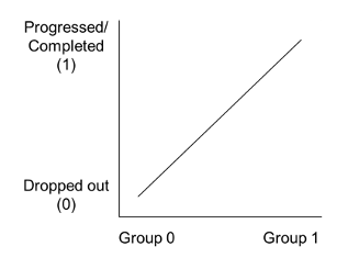
Figure 4. Visual depiction of a positive relationship between student background group and continuation
The question we aim to answer in this tutorial is: Is there a continuation gap based on the students’ background groups, and can a set of micro-level factors predict continuation over and above these groups? For Tutorial 2, we performed a binary logistic regression analysis to determine the relative contribution that each variable might make to explaining the odds of students dropping out of university or progressing/completing. We began by specifying the models, so in the first model we entered the student background group variable on its own (Model 1). We then entered prior attainment, entry qualification, and the measure of belonging into the next model (Model 2). The Individual_Level_Continuation.sps SPSS syntax file includes the code for all stages of this analysis. Findings from model specifications are found in Figure 5.
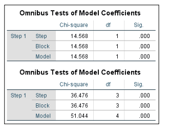
Figure 5. SPSS output of model summary tables from models 1 (table above) and 2 (table below) in logistic regression analysis of Individual_Level_Example.sav data set using Individual_Level_Continuation.sps syntax
Figure 5 demonstrates whether each model is a good fit to the data. The Model row of the first table indicates that Model 1 (which includes the student background group variable only) is a significant fit to the data (p < .001). The Block row in the second table indicates that the change from Model 1 to Model 2 (which adds all covariates) is significant (p < .001). As with Tutorial 1, we need to check for any sources of bias in the data (i.e. outliers and influential cases), and whether certain assumptions have been met if we want to generalise the model. Diagnostic tests for checking sources of bias and whether assumptions have been met have been included in the SPSS syntax. We now look at the contribution each individual covariate made to each model by examining the Variables in the Equation tables from the SPSS Output (Figure 6).
Figure 6. SPSS output of variables in the equation tables from models 1 (table above) and 2 (table below) in logistic regression analysis of Individual_Level_Example.sav data set using Individual_Level_Continuation.sps syntax
The tables in Figure 6 show the individual contribution of each covariate to each model in the analysis. All B-values indicate positive relationships and are significant, but the OR values (labelled as Exp(B) in the SPSS output) are easier to interpret. In Model 1, the OR for student background group is 6.449. This value is greater than one, which indicates a positive relationship between student background group and continuation, and this is significant (p < .001). Therefore, students coded as group 0 were more likely to drop out (also coded as 0) than students coded as group 1 by a factor of 6.449. In other words, students coded as group 0 were over six times as likely to drop out than students coded as group 1, demonstrating that a continuation gap is present. In Model 2, the effect of background group drops to non-significance (p = .123, and the confidence interval, labelled as 95% C.I. for EXP(B) in the SPSS output, also crosses one) and prior attainment is also non-significant (p = .072). Entry qualification and sense of belonging are significant (OR = 7.785, p < .001 and OR = 2.208, p = .018, respectively). This indicates that students with lower scores on the measure of belonging and Qualification type A (coded as 0) were more likely to drop out (also coded as 0), assuming the effects of all other variables are held constant. Finally, we can check for interdependence between covariates by checking whether covariates are correlated, and whether there is evidence of multicollinearity by running a linear regression analysis (included in the SPSS syntax) to check tolerance and VIF values.
In this example, we aimed to determine whether there were continuation gaps based on students’ background groups, and whether a set of micro-level factors could predict continuation over and above these groups. The analysis of this hypothetical data set indicates that students coded as group 0 were more likely to drop out than students coded as group 1. However, this association was not present once taking into account students’ entry qualification and their sense of belonging to the university, which better predicted the odds of students dropping out or progressing/completing.
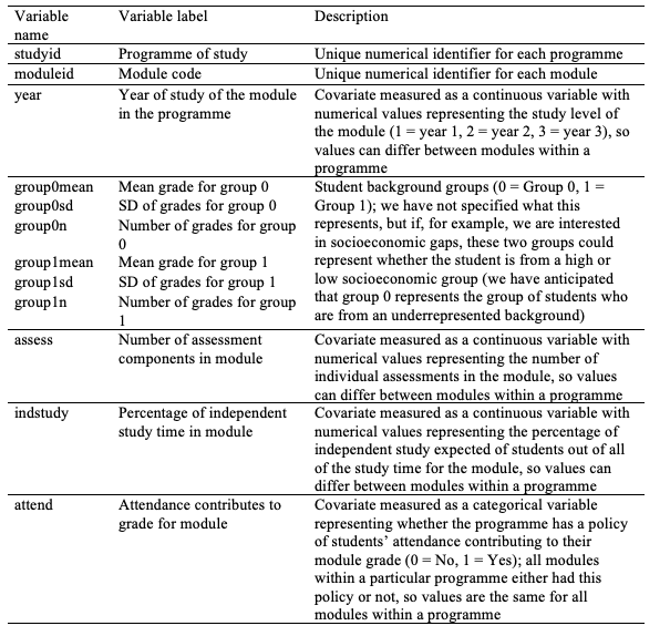
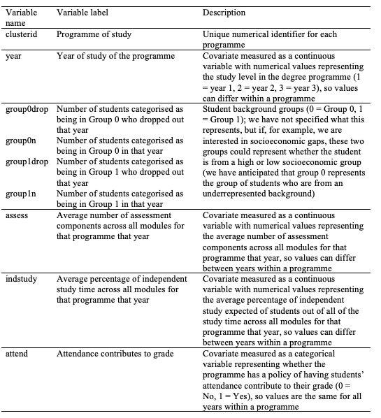
Tutorial 3 presents an analysis of the Group_Level_Attainment_Example.sav SPSS data set, which was designed to closely approximate what real aggregated student data might look like when modelling attainment gaps. This hypothetical data set simulates a range of variables for a sample of 1056 modules within 40 programmes. The variables are detailed in Table 3 and include: Average grades at a module-level for two different groups of students (student background group), the year of study of the module in the programme, and a set of meso-level variables that may account for differential student outcomes (as influenced by theory) to be used as covariates.
When modelling attainment gaps at an individual level (Tutorial 1), the outcome was students’ grades and the initial covariate entered in the analysis was the student background group variable. Extending this to a group level, the difference in average grades between the two groups for a particular module represents an effect size 5 , so this is our outcome variable when using meta-regression. Standard meta-analytic techniques are predicated on the assumption that effect sizes are independent (Cheung, 2019). However, effect sizes for each module are likely to be dependent because grades for each module will include the same students across a programme, known as correlated effects (Hedges et al., 2010; Tipton & Pustejovsky, 2015). Robust variance estimation (RVE) can be used in meta-regression analyses to correct for correlated estimates (Hedges et al., 2010)6 . Meta-analyses using RVE with fewer than 40 studies may produce overly narrow confidence intervals (Tanner-Smith & Tipton, 2014), so we recommend that analyses include at least 40 programmes. 7 Consideration should also be given to the inclusion of modules with very few students from a particular background group, because effect sizes based on small sample sizes could artificially inflate the size of gaps. One way to check for this is to perform sensitivity analyses, which involves running analyses with and without the data from particular modules to see whether their inclusion appears to bias the results.
Since we are focusing on explaining the attainment gaps themselves, the question we aim to answer in this tutorial is: Are there attainment gaps based on the students’ background groups, and can a set of meso-level factors predict these gaps? For Tutorial 3, we performed a meta-regression analysis using RVE with correlated effects weights. The background group variable does not need to be entered into the analysis as a separate variable, so no covariates were included in the first model. This intercept-only model therefore tested whether there was a significant attainment gap between the two student groups (Model 1), equivalent to the first model in Tutorial 1. Before entering any of the covariates 8 into the analysis we needed to code whether values of covariates can differ within a programme (i.e. values differ between modules within a programme) or only between programmes (i.e. values are the same for all modules within a programme). In the current example, the attendance variable could only differ between programmes (i.e. all modules within a programme took on the same value), so this variable could be included in the analysis as it is. However, the following covariates had the potential to take on different values across modules within a single programme: Year of study of the module in the programme (because each programme included modules across years 1, 2 or 3), number of assessment components, and percentage of independent study time expected of students. Therefore, new variables needed to be created in SPSS to average the scores for these covariates across all modules within a programme (programme-mean values for each variable to model between-programme effects) and to center these covariate scores around the programme-mean (to model within-programme/between-module effects). This is an important step, because it separates out between- and within-effects to aid the interpretation of covariate effects (Tanner-Smith & Tipton, 2014). We then entered all covariates into Model 29. These included: Year of study of the module, number of assessment components, the percentage of independent study time, and the attendance variable. We also needed to specify a rho value to represent the estimated size of intercorrelations expected between effect sizes within a programme. Rho values range between 0 and 1, with higher values indicating greater dependence. As this value is only an estimate of dependency, we used a conservative rho value of .80.
Table 3
Variables included in Group_Level_Attainment_Example.sav SPSS data set
The Group_Level_Attainment.sps SPSS syntax file includes the code for all stages of this analysis, including the creation of new covariate variables with centered and mean scores. The freely available RVE meta-regression SPSS macro file, RobustMeta.sps (Tanner-Smith & Tipton, 2014)10 , should be saved on the computer that will be used for performing analyses prior to running any SPSS syntax files, and the file path for where this macro is saved needs to be added to the syntax, as noted in the syntax instructions. Figure 7 displays the SPSS output for the model that did not include any covariates.
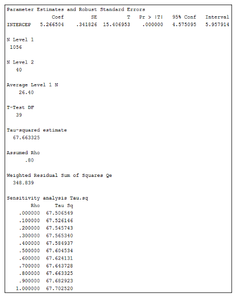
Figure 7. SPSS output of the intercept-only model (Model 1) from meta-regression analysis of Group_Level_Attainment_Example.sav data set using Group_Level_Attainment.sps syntax
In Figure 7, the B-value for the constant (labelled as Coef in the SPSS output) is 5.27, which represents the overall effect size (i.e. attainment gap) across all modules, and this is significant (p < .001; significance is labelled as Pr > |T| in the SPSS output). Because this value was calculated by deducting the average grade of Group 0 from the average grade of Group 1, we can ascertain that the positive mean difference indicates that Group 1 has a higher average grade (5.27% greater) than Group 0, demonstrating that an attainment gap is present. The N Level 1 value shows that 1056 effect sizes were included in the analysis and the N Level 2 value shows that there were 40 programmes. The Average Level 1 N value shows that there was an average of 26.40 modules per programme in the analysis. The Assumed Rho of .80 is the average intercorrelation we expected there to be between module effect sizes. Finally, the Tau-squared estimate indicates the amount of variance between programmes at the rho level we selected, and the sensitivity analysis shows how this amount of variance would have differed at different rho levels. We can see from this range that the variance level would not have been that different if we expected there to be a smaller or larger intercorrelation between modules. Model 2 is displayed in Figure 8.
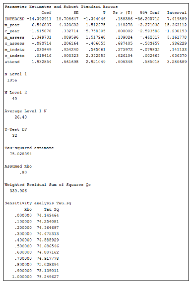
Figure 8. SPSS output of Model 2 from meta-regression analysis of Group_Level_Attainment_Example.sav data set using Group_Level_Attainment.sps syntax
Figure 8 includes all of the covariates in the meta-regression analysis. The m_ (mean) prefix denotes that values for this variable have been averaged within a programme to allow us to interpret between-programme effects, whereas the c_ (center) prefix denotes that these variables have been centered around the programme-mean to reflect within-programme (or between-module) effects. Firstly, year of study is a significant negative covariate within programmes (labelled c_year in the SPSS output; p < .001), which means that the size of any attainment gaps decreases as students transition through university. The amount of independent study time expected of students is also a significant positive covariate within programmes (labelled c_indstu in the SPSS output; p = .026), with the size of attainment gaps increasing as the amount of expected independent study time increases. Finally, the attendance variable is a significant positive covariate (labelled attend in the SPSS output; p = .006), so having a policy of attendance contributing to students’ grades (coded as 1) predicts a larger gap in attainment between groups. As with the regression analysis in Tutorial 1, the B-values in the Coef column can also be used to understand how much change we would expect in the attainment gap from a one unit change in these variables (based on whatever units the original variables were measured in), whilst holding the effects of all other variables constant. In this example, we aimed to determine whether there were attainment gaps based on students’ background groups, and whether a set of meso-level factors could predict these gaps. The analysis of this hypothetical data set indicates that students coded as group 1 performed better than students coded as group 0, and this overall attainment gap can be explained by the year of study of the module, the amount of independent study time expected of students in the module, and whether there is a policy of attendance contributing to students’ grades.
Tutorial 4 presents an analysis of the Group_Level_Continuation_Example.sav SPSS data set, which was designed to closely approximate what real aggregated student data might look like when modelling continuation gaps. Continuation occurs at the year-level (rather than at a module-level) within a programme; students either progress from one year to the next (and then complete their studies) or drop out. Therefore, this hypothetical data set simulates a range of variables for a sample of 40 programmes, split by the year of study of the programme. The data set includes the number of students who dropped out of university during a particular year of study for two different groups of students (student background group). It also includes the same set of meso-level variables used as covariates in Tutorial 3, instead averaged across all modules for the year of the programme rather than split by module (the variables are detailed in Table 4).
There are three types of effect size that could be calculated for these data set for use in the meta-regression analysis. The first effect size option is to calculate the risk ratio, which in this example would be the ratio between the risk of dropout for one student group compared to the risk of dropout for the other group. The second effect size option is to calculate the risk difference, which is the difference between these two risks. The final option is to calculate the OR, which is what is used in logistic regression analyses. Hedges et al. (2009) suggest that ORs have statistical properties that often make them the best effect size option with meta-analyses of binary data, so since this statistic was also used when modelling continuation gaps at an individual level (Tutorial 2), we have used it with the current data in this tutorial. However, the SPSS syntax for this example also computes variables for risk ratios and risk differences in case the reader would prefer to use these measures instead. It is also necessary to use the log-transformed OR over the raw OR to ensure that there is a balance in ratios between groups (Hedges et al., 2009). When modelling continuation gaps at an individual level (Tutorial 2), the outcome was the continuation variable and the initial covariate entered in the analysis was the student background group variable. Extending this to a group level, the log OR for the association between these two variables (see Table 2) represents an effect size, so this is our outcome variable when using meta-regression.
Table 4
Variables included in Group_Level_Continuation_Example.sav SPSS data set
The Group_Level_Continuation_Example.sav SPSS data set includes the dropout numbers for each year of a programme (i.e. years 1, 2 and 3) at a single point in time. Therefore, unlike the data set used in Tutorial 3, effect sizes do not include any of the same students. However, whilst effect sizes are independent, there are three separate effect sizes clustered within each programme (one for each year of students’ study). Therefore, there may be hierarchical dependence between effect sizes (Tipton & Pustejovsky, 2015), because although different individuals contribute to each effect size, there may be a shared influence on patterns of continuation within a particular programme (e.g. because the same staff may teach across years on a programme, there may be similarities in curriculum design across a programme, etc.). It is worth noting that hierarchical dependency may also have been present in the data set used for Tutorial 3, since each programme was also clustered within a department/school that may have led to shared influences between programmes. However, it has been advised that the analysis should use the weights (correlated or hierarchical) based on the most common type of dependency in the data (Tanner-Smith et al., 2016; Tipton & Pustejovsky, 2015).
Since we are focusing on explaining the continuation gaps themselves, the question we aim to answer in this tutorial is: Are there continuation gaps based on the students’ background groups, and can a set of meso-level factors predict these gaps? For Tutorial 4, we performed a meta-regression analysis using RVE with hierarchical effects weights. The background group variable does not need to be entered into the analysis as a separate variable, so no covariates were included in the first model. This intercept-only model therefore tested the odds that students in one group were more likely to drop out (Model 1), equivalent to the first model in Tutorial 2. As with Tutorial 3, new variables needed to be created to average covariates across all modules within a programme (programme-mean values for each variable to model between-programme effects) and to center these variables around the programme-mean (to model within-programme/between-year effects), so this was done for the number of assessments and percentage of independent study time variables. We then entered year of study, the average number of assessment components, and the average percentage of independent study time into the next model (Model 2). The Group_Level_Continuation.sps SPSS syntax file includes the code for all stages of this analysis, and again, the SPSS macro file, RobustMeta.sps (Tanner-Smith & Tipton, 2014), needs to be saved on the computer that will be used for performing analyses prior to running any SPSS syntax files, and the file path for where this macro is saved needs to be added to the syntax, as noted in the syntax instructions. Figure 9 displays the SPSS output for the model that did not include any covariates.
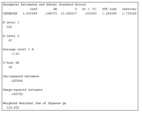
Figure 9. SPSS output of the intercept-only model (Model 1) from meta-regression analysis of Group_Level_Continuation_Example.sav data set using Group_Level_Continuation.sps syntax
In Figure 9, the B-value for the constant is 1.54, which represents the overall log OR across all years. This effect size is positive and statistically significant (p < .001). As each OR is calculated based on the coding used in Table 2, the positive value for the effect size indicates that students coded as group 0 were more likely to drop out than students coded as group 1, demonstrating that a continuation gap is present. We can convert this back to a raw OR by using an exponential function (e.g. the Excel formula =EXP), which gives an OR value of 4.67. The OR value greater than one indicates that students coded as group 0 were more likely to drop out than students coded as group 1 by a factor of 4.67. In other words, students coded as group 0 were over four times as likely to drop out than students coded as group 1. The N Level 1 value shows that 120 effect sizes were analysed, and the N Level 2 value shows that there were 40 programmes. The Average Level 1 N value shows that there was an average of three years of study per programme in the analysis. Finally, the Tau-squared estimate indicates the amount of variance between programmes, and the Omega-square estimate indicates the amount of variance between years within programmes. Model 2 is displayed in Figure 10.
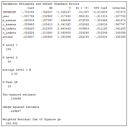
Figure 10. SPSS output of Model 2 from meta-regression analysis of Group_Level_Continuation_Example.sav data set using Group_Level_Continuation.sps syntax
Figure 10 includes all of the covariates in the meta-regression analysis. As was done in Tutorial 3, variables with an m_ prefix have been averaged within a programme to allow us to interpret between-programme effects, and variables with a c_ prefix have been centered around the programme-mean to reflect within-programme (or between-year) effects. Firstly, the number of assessments is a significant positive covariate within programmes (labelled c_assess in the SPSS output; p = .002). Since the effect size has been computed as per the coding in Table 2 (with a higher number indicating that students coded as group 0 have a higher chance of dropping out), this means that as the number of assessment components increases, so do the odds of students coded as group 0 dropping out. The amount of independent study time expected of students is also a significant positive covariate both between programmes (labelled m_indstu in the SPSS output; p = .006) and within programmes (labelled c_indstu in the SPSS output; p = .024), meaning that as the amount of expected independent study time increases, so do the odds of students coded as group 0 dropping out. If the B-values are converted to ORs, they can also be used to understand the likelihood to dropout occurring based on a one unit change in these variables, whilst holding the effects of all other variables constant.
In this example, we aimed to determine whether there were continuation gaps based on students’ background groups, and whether a set of meso-level factors could predict these gaps. The analysis of this hypothetical data set indicates that students coded as group 0 were more likely to drop out than students coded as group 1, and this overall continuation gap can be explained by the average number of assessment components and the average amount of independent study time expected of students.
The purpose of this primer is not to encourage teaching staff to make large-scale changes to their practice based on evidence from quantitative analyses of institutional data alone. We believe this would be very ill-advised for reasons we will now discuss. Most importantly, if data are gathered and analysed in the ways demonstrated in this primer, any associations between covariates and outcomes are not causal, so we cannot claim that these micro- and meso-level factors are causing any observed gaps. Analyses should also be driven by theory, so variables should not simply be included just because data are available, as this may lead to false positives. Of course, there is an opportunity to incorporate variables in analyses in an exploratory sense in order to extend the evidence-base on explanatory factors, but efforts should be made to avoid the “tendency to constantly extend the data inquiry to look at more variables with diminishing returns in terms of understanding” (Mountford-Zimdars et al., 2015, p. 22). Furthermore, an explanatory factor in one area might not be the case in other areas, which limits the generalisability of analyses unless it can be argued that student populations are equivalent and representative. This is why interventions may not always prove to be successful across contexts.
There is also the risk of potential biases in interpretations occurring that readers should attempt to avoid. Firstly, as noted above, each time a covariate is added to a GLM analysis, the coefficients for other covariates change (unless there is zero correlation between covariates, which is unlikely), so each model is context-specific (Dunlap & Landis, 1998). ORs (see Tutorials 2 and 4) cannot be compared across models for this same reason (Mood, 2010). High interdependence between covariates can also be problematic, so Karpen (2017) suggests the use of relative importance analysis, which transforms covariates so they become uncorrelated, as an alternative to linear regression in these situations. Tonidandel and LeBreton (2015) produced a free web-based tool for performing relative importance analyses. Secondly, if readers make the assumption that associations found at the group level apply to the individuals within such groups, they will encounter the ecological fallacy (Freedman, 1999). If an analysis of this same data at an individual level leads to different findings, ecological bias has occurred. Tutorials 3 and 4 show how analyses of aggregated data can enable the introduction of group-level (i.e. meso- and macro-level) variables, which are not able to be incorporated into the individual-level analyses in Tutorials 1 and 2. Because meso- and macro-level explanatory factors manifest at the group level, these variables are not simply individual-level variables that have been aggregated. Therefore, we were not attempting to draw micro-level conclusions about individuals with aggregated data, so we should not be committing the ecological fallacy, because the group level is the level of interest (Schwartz, 1994). However, readers should be careful to avoid simply aggregating individual-level covariates for use with aggregated student data in order to avoid committing this fallacy. Finally, we do not see the discussed approaches to gathering and analysing quantitative evidence as replacing rich qualitative research on differential student outcomes. Qualitative data may be needed to make sense of what the quantitative findings show. For example, if a factor is strongly associated with the presence of gaps, focus groups could be held with students and teaching staff in areas where that factor is particularly prevalent to learn more about the mechanisms impacting on that factor. As a result of the discussed issues, these analyses alone could never tell the complete story, so we advise that results only be used to highlight specific variables of interest for further investigation or to focus the design of novel interventions.
We anticipate that the guidance presented in this primer can enable universities to take a more proactive approach to monitoring and reducing gaps. Gathering data on explanatory factors to which many institutions already have access, and integrating these with existing institutional data on differential outcomes, can only enhance the sophistication of any analyses. To elucidate this point, we can look at the hypothetical findings of the four illustrative examples; although they do not draw on real data, if the findings were real we could conclude that attainment and continuation gaps are present in the data sets and a range of micro- and meso-factors can account for these gaps, including students’ entry qualification, prior attainment, their sense of belonging to the university, their year of study, the amount of independent study time expected of them, and whether there is a policy of attendance contributing to their grades. In relation to the conceptual model in Figure 1, these findings would highlight the specific aspects of curriculum and assessment factors that play a role in differential outcomes, rather than only viewing this in terms of the broad categories of ‘curriculum’ and ‘assessment’. The meta-regression techniques are also novel and parsimonious ways of directly analysing attainment and continuation gaps using aggregated data that avoid issues with data privacy. As a result, we believe this primer will be of particular interest to staff with strategic responsibilities who report on the presence of gaps within their institution. Our guidance should raise awareness around the causes of differential outcomes and enable these staff to provide teaching staff with more nuanced evidence that can be used for focusing conversations around issues that have been identified and designing context-specific interventions, whether these are universal or targeted at specific student groups. For example, based on the hypothetical findings from the illustrative examples, teaching staff might decide to speak with students about how they feel about the balance of independent study time in their modules and any policies around attendance contributing to their grades. Interventions might then be designed based on these aspects of the curriculum and assessment. This evidence is likely to be relevant to specific modules/programmes/disciplines, so rather than just replicating current interventions that may only be effective within specific contexts, findings from analyses could increase institutions’ understanding about the factors that are salient for their own students. This increased precision in the evidence-base used for designing novel interventions means that there will be less investment in approaches that are not likely to work. Implementation of the suggested analyses thus represents better value for money in any initiatives undertaken by institutions. Furthermore, this will also assuage deficit assumptions that differential outcomes are due to student deficiencies, which could be used to excuse teaching staff from their own responsibilities for attempting to tackle gaps.
Although this primer particularly attends to opportunities for exploring meso-level variables, largely because these variables are under the control of the university, there is the potential for analysing cross-institutional data, possibly internationally, to consider the role of quantitative macro-level explanatory factors in differential student outcomes. Meta-regression techniques in particular may support these endeavours, since there are likely to be far fewer issues sharing aggregated data between institutions than there would be with individual-level data. Additionally, if metrics for attainment and continuation are different between institutions, it is possible to standardise them for comparison using these techniques. Cross-institutional comparisons would enable a better understanding of how institution type and context impact on gaps.
Finally, beyond the practical implications discussed, an important contribution of this primer for researchers is that it provides them with methods to extend the literature on differential outcomes, potentially uncovering new insights about multi-level causes of attainment and continuation gaps. One way researchers could do this is by considering how to operationalise some of the micro- and meso-level factors in the conceptual model in Figure 1 that have not previously been quantitatively measured and analysed. For example, data on research income and research and teaching quality metrics could be used as measures of institutional and disciplinary culture (see Boliver, 2015, for an analysis of publicly available data encompassing these variables). This approach may then call attention to the specific facets of the conceptual model that merit closer scrutiny in future research. Depending on the representativeness of the student populations investigated, potential future research using the approaches in this primer might also consider how meso-level factors manifest differently based on variation in macro-level factors, and how micro-level factors differ based on variation in meso-level factors. For instance, macro-level factors, such as the structure and hierarchy of an institution could affect the design of its learning environments at the meso-level (e.g. teaching-led universities might prioritise innovative teaching approaches more than research-intensive institutions), so moderating effects between micro-, meso-, and macro-level variables on gaps could be explored. As previously noted, differential student outcomes are quantitatively assessed (Jones, 2018), so if researchers adopt the quantitative methods used in this primer, they could reveal more about the explanatory power of specific factors, which could enrich the largely qualitative evidence-base. Furthermore, by revealing more about potential predictors of gaps, the methods could also open up new conversations with students, providing fresh avenues for future qualitative research in this area. Therefore, this primer offers significant scope for developing theoretical perspectives on differential outcomes beyond current understandings in the literature. It is only by fully exploring potential causes of gaps at all levels that we will fully understand the role of student diversity in educational transitions.
The authors thank Professor Chris Fife-Shaw, Dr Anesa Hosein, Nicholas Moore and Dr James Munro for their insightful comments on earlier drafts of this manuscript.
1 Throughout this primer we refer to different aspects of university based on terminology usually used in the UK higher education context (e.g. degree courses are referred to as programmes, subject units are referred to as modules, etc.).
2 All analyses can also be performed using other software packages, such as Stata and R, so .csv files (for the data sets) and .txt files (for the syntax) have additionally been provided to enable readers to adapt these files for use with their preferred software.
3 Our use of the term covariate is synonymous with predictor/independent variable (or moderator in meta-analyses).
4 Binary/dichotomous variables (i.e. variables with only two categories) can be entered into regression models as covariates and treated the same as continuous variables if they are coded as 0 and 1. However, categorical variables with more than two categories need to be converted into a set of binary variables, known as dummy coding, before inclusion. Field (2018, pp. 509–516) provides an accessible overview of dummy coding.
5 If different measures of attainment are used (e.g. combining grade percentages with grade point average), or if the measure of attainment is not meaningful (e.g. the attainment metric is specific to a particular institution), the standardised difference in means should be used as the effect size measure instead of the raw difference (Hedges et al., 2009); code for computing standardised effect sizes has been included in the SPSS syntax file.
6 RVE can also be performed in R using the robumeta package (Fisher et al., 2017; see Tanner-Smith et al., 2016, for a tutorial), and in Stata using the robumeta.ado macro (see Tanner-Smith & Tipton, 2014, for syntax and a tutorial).
7 Small-sample adjustments in RVE are not available in the SPSS macro, but they are part of the Stata macro and R package for RVE (Tanner-Smith et al., 2016).
8 The degrees of freedom in RVE analyses are constrained by the number of studies (in this case, the number of programmes) being analysed, not the number of effect sizes (Tanner-Smith & Tipton, 2014). Therefore, readers should be cautious about including too many covariates in analyses with only a limited number of programmes being analysed.
9 As with regression analyses performed on individual-level data, it is possible to check for sources of bias, meeting of assumptions, and issues with multicollinearity. However, more sophisticated software is needed for these tests than the SPSS macro used for tutorials 3 and 4, so findings should be interpreted with some caution in the absence of these tests.
10 This macro has also been converted into an SPSS plug-in to enable analyses to be run through the main SPSS menus. This can be downloaded from https://github.com/ahmaddaryanto/meta_analysis_SPSS_Macros.
Alin, A. (2010). Multicollinearity.Wiley Interdisciplinary
Reviews: Computational Statistics, 2(3), 370–374.
https://doi.org/10.1002/wics.84
Boliver, V. (2015). Are there distinctive clusters of higher and
lower status universities in the UK? Oxford Review of
Education, 41(5), 608–627.
https://doi.org/10.1080/03054985.2015.1082905
Broecke, S., & Nicholls, T. (2007). Ethnicity and degree
attainment (DfES Research Report RW92). DfES.
Cheung, M. W. L. (2019). A guide to conducting a meta-analysis
with non-independent effect sizes. Neuropsychology Review,
29 (4), 387–396.
https://doi.org/10.1007/s11065-019-09415-6
Courville, T., & Thompson, B. (2001). Use of structure
coefficients in published multiple regression articles: β is not
enough. Educational and Psychological Measurement, 61(2),
229–248. https://doi.org/10.1177/0013164401612006
Cousin, G., & Cuerton, D. (2012). Disparities in student
attainment (DISA). Higher Education Academy (HEA).
https://www.advance-he.ac.uk/knowledge-hub/disparities-student-attainment
Dunlap, W. P., & Landis, R. S. (1998). Interpretations of
multiple regression borrowed from factor analysis and canonical
correlation. The Journal of General Psychology, 125(4),
397–407. https://doi.org/10.1080/00221309809595345
Field, A. P. (2018). Discovering statistics using IBM SPSS
Statistics (5th ed.). Sage.
Field, A. P., & Gillett, R. (2010). How to do a meta-analysis.British
Journal of Mathematical and Statistical Psychology, 63(3),
665–694. https://doi.org/10.1348/000711010X502733
Fisher, Z., Tipton, E., & Zhipeng, H. (2017). robumeta
(Version 2.0) [Computer software].
https://cran.r-project.org/package=robumeta
France, M. K., Finney, S. J., & Swerdzewski, P. (2010).
Students’ group and member attachment to their university: A
construct validity study of the University Attachment Scale. Educational
and Psychological Measurement, 70(3), 440–458.
https://doi.org/10.1177/0013164409344510
Freedman, D. A. (1999). Ecological inference and the
ecological fallacy (Technical Report 549) .
https://statistics.berkeley.edu/sites/default/files/tech-reports/549.pdf
Gravett, K. (2019). Troubling transitions and celebrating
becomings: from pathway to rhizome. Studies in Higher
Education, 1–12.
https://doi.org/10.1080/03075079.2019.1691162
Hedges, L. V., Borenstein, M., Higgins, J. P. T., & Rothstein,
H. R. (2009). Introduction to meta-analysis. John Wiley
& Sons, Ltd.
Hedges, L. V., Tipton, E., & Johnson, M. C. (2010). Robust
variance estimation in meta-regression with dependent effect size
estimates. Research Synthesis Methods, 1(1),
39–65. https://doi.org/10.1002/jrsm.5
Jones, S. (2018). Expectation vs experience: might transition gaps
predict undergraduate students’ outcome gaps? Journal of
Further and Higher Education, 42(7), 908–921.
https://doi.org/10.1080/0309877X.2017.1323195
Karpen, S. C. (2017). Misuses of regression and ANCOVA in
educational research. American Journal of Pharmaceutical
Education, 81(8), 84–85.
https://doi.org/10.5688/ajpe6501
Lens, D., & Levrau, F. (2020). Can pre-entry characteristics
account for the ethnic attainment gap? An analysis of a Flemish
university. Research in Higher Education, 61(1),
26–50. https://doi.org/10.1007/s11162-019-09554-y
Miller, M. (2016). The ethnicity attainment gap: literature
review . The University of Sheffield Widening Participation
Research & Evaluation Unit.
https://www.sheffield.ac.uk/polopoly_fs/1.661523!/file/BME_Attainment_Gap_Literature_Review_EXTERNAL_-_Miriam_Miller.pdf
Mood, C. (2010). Logistic regression: Why we cannot do what we
think we can do, and what we can do about it. European
Sociological Review, 26(1), 67–82.
https://doi.org/10.1093/esr/jcp006
Mountford-Zimdars, A., Sabri, D., Moore, J., Sanders, J., Jones,
S., & Hiagham, L. (2015). Causes of differences in
student outcomes. Higher Education Funding Council for
England (HEFCE).
https://webarchive.nationalarchives.gov.uk/20180405123119/http://www.hefce.ac.uk/pubs/rereports/Year/2015/diffout/
Mountford-Zimdars, A., Sanders, J., Moore, J., Sabri, D., Jones,
S., & Higham, L. (2017). What can universities do to support
all their students to progress successfully throughout their time
at university? Perspectives: Policy and Practice in Higher
Education, 21 (2–3), 101–110.
https://doi.org/10.1080/13603108.2016.1203368
OfS. (n.d.). Continuation and attainment gaps.
https://www.officeforstudents.org.uk/advice-and-guidance/promoting-equal-opportunities/evaluation-and-effective-practice/continuation-and-attainment-gaps/
Pigott, T. D., & Polanin, J. R. (2020). Methodological
guidance paper: High-quality meta-analysis in a systematic review.
Review of Educational Research, 90(1), 24–46.
https://doi.org/10.3102/0034654319877153
Schwartz, S. (1994). The fallacy of the ecological fallacy: the
potential misuse of a concept and the consequences. American
Journal of Public Health, 84(5), 819–824.
https://doi.org/10.2105/AJPH.84.5.819
Singh, G. (2011). Black and Minority Ethnic (BME) students
participation in higher education: improving retention and
success . Higher Education Academy (HEA).
https://www.heacademy.ac.uk/system/files/bme_synthesis_final.pdf
Stevenson, J. (2012). Black and minority ethnic student
degree retention and attainment. Higher Education Academy
(HEA).
https://www.heacademy.ac.uk/system/files/bme_summit_final_report.pdf
Tanner-Smith, E. E., & Tipton, E. (2014). Robust variance
estimation with dependent effect sizes: practical considerations
including a software tutorial in Stata and SPSS. Research
Synthesis Methods, 5 (1), 13–30.
https://doi.org/10.1002/jrsm.1091
Tanner-Smith, E. E., Tipton, E., & Polanin, J. R. (2016).
Handling complex meta-analytic data structures using robust
variance estimates: a tutorial in R. Journal of Developmental
and Life-Course Criminology, 2 (1), 85–112.
https://doi.org/10.1007/s40865-016-0026-5
Thompson, C. G., Kim, R. S., Aloe, A. M., & Becker, B. J.
(2017). Extracting the Variance Inflation Factor and other
multicollinearity diagnostics from typical regression results. Basic
and Applied Social Psychology, 39(2), 81–90.
https://doi.org/10.1080/01973533.2016.1277529
Tieben, N. (2020). Non-completion, transfer, and dropout of
traditional and non-traditional students in Germany. Research
in Higher Education, 61(1), 117–141.
https://doi.org/10.1007/s11162-019-09553-z
Tinto, V. (1993). Leaving college: Rethinking the causes and
cures of student attrition (2nd ed.). University of
Chicago Press.
Tipton, E., & Pustejovsky, J. E. (2015). Small-sample
adjustments for tests of moderators and model fit using robust
variance estimation in meta-regression. Journal of
Educational and Behavioral Statistics, 40(6),
604–634. https://doi.org/10.3102/1076998615606099
Tonidandel, S., & LeBreton, J. M. (2015). RWA Web: A free,
comprehensive, web-based, and user-friendly tool for relative
weight analyses. Journal of Business and Psychology, 30(2),
207–216. https://doi.org/10.1007/s10869-014-9351-z
UUK & NUS. (2019). Black, Asian and minority ethnic
student attainment at UK universities: #closingthegap .
Universities UK & National Union of Students.
https://www.universitiesuk.ac.uk/news/Pages/Universities-acting-to-close-BAME-student-attainment-gap.aspx
Woodfield, R. (2014). Undergraduate retention and attainment
across the disciplines. Higher Education Academy (HEA).
https://www.advance-he.ac.uk/knowledge-hub/undergraduate-retention-and-attainment-across-disciplines